Decision Tree
Classification is a two-step process, learning step and prediction step, in machine learning. In the learning step, the model is developed based on given training data. In the prediction step, the model is used to predict the response to given data. Decision Tree is one of the easiest and most popular classification algorithms to understand and interpret.
Decision Tree Algorithm
The decision Tree algorithm belongs to the family of supervised learning algorithms. Unlike other supervised learning algorithms, the decision tree algorithm can be used for solving regression and classification problems too.
The goal of using a Decision Tree is to create a training model that can use to predict the class or value of the target variable by learning simple decision rules inferred from prior data (training data).
In Decision Trees, for predicting a class label for a record we start from the root of the tree. We compare the values of the root attribute with the record’s attribute. On the basis of comparison, we follow the branch corresponding to that value and jump to the next node.
Types of Decision Trees
Types of decision trees are based on the type of target variable we have. It can be of two types:
- Categorical Variable Decision Tree: A decision Tree that has a categorical target variable then it called a Categorical variable decision tree.
- Continuous Variable Decision Tree: A decision Tree has a continuous target variable then it is called Continuous Variable Decision Tree.
Example: – Let’s say we have a problem predicting whether a customer will pay his renewal premium with an insurance company (yes/ no). Here we know that the income of customers is a significant variable but the insurance company does not have income details for all customers. Now, as we know this is an important variable, then we can build a decision tree to predict customer income based on occupation, product, and various other variables. In this case, we are predicting values for the continuous variables.
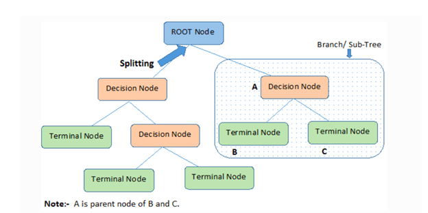
Important Terminology Related to Decision Trees
- Root Node: It represents the entire population or sample and this further gets divided into two or more homogeneous sets.
- Splitting: It is a process of dividing a node into two or more sub-nodes.
- Decision Node: When a sub-node splits into further sub-nodes, then it is called the decision node.
- Leaf / Terminal Node: Nodes that do not split are called Leaf or Terminal Node.
- Pruning: When we remove sub-nodes of a decision node, this process is called pruning. You can say the opposite process of splitting.
- Branch / Sub-Tree: A subsection of the entire tree is called a branch or sub-tree.
- Parent and Child Node: A node, which is divided into sub-nodes is called a parent node of sub-nodes whereas sub-nodes are the child of a parent node.
Assumptions while Creating Decision Tree
Below are some of the assumptions we make while using the Decision tree:
- In the beginning, the whole training set is considered as the root.
- Feature values are preferred to be categorical. If the values are continuous then they are discretized prior to building the model.
- Records are distributed recursively on the basis of attribute values.
- Order to place attributes as root or internal nodes of the tree is done by using some statistical approach.
Attribute Selection Measures
If the dataset consists of N attributes then deciding which attribute to place at the root or at different levels of the tree as internal nodes is a complicated step. By just randomly selecting any node to be the root can’t solve the issue. If we follow a random approach, it may give us bad results with low accuracy.
For solving this attribute selection problem, researchers worked and devised some solutions. They suggested using some criteria like:
- Entropy,
- Information gain,
- Gini index,
- Gain Ratio,
- Reduction in Variance
- Chi-Square
These criteria will calculate values for every attribute. The values are sorted, and attributes are placed in the tree by following the order i.e., the attribute with a high value (in case of information gain) is placed at the root. While using Information Gain as a criterion, we assume attributes to be categorical, and for the Gini index, attributes are assumed to be continuous.